Blog 27 – Estimands Part 3B – What Is the ITT Estimand Anyway?

Introduction

This is part of a series of Blogs on the topic of estimands. It originates with the publication of “ICH E9 (R1) addendum on estimands and sensitivity analysis in clinical trials to the guideline on statistical principles for clinical trials.” [ICH, 2019] Henceforth this will be referred to as the Addendum. The guideline mentioned in that title is in fact “ICH E9 Statistical Principles for Clinical Trials.” [ICH, 1998] Since the publication of ICH E9(R1), the Addendum, there have been multitudinous conversations in the statistical community, as well as some in the clinical community – through publications, conferences, training materials etc. – related to the implementation of the “estimand framework” for regulated clinical research. Suffice to say, the implementation has hit some bumps in the road, and this Blog is in specific response to a recently published paper on the topic – “A Perspective on the Appropriate Implementation of ICH E9(R1) Addendum Strategies for Handling Intercurrent Events.” [Fleming, 2025]. Henceforth merely referred to as Fleming.

The reader of this Blog is encouraged to read Blog 24 (some history on ITT), Blog 25 (what an estimand is) and Blog 26 (what is the question?) as background for this ongoing series of Blogs. This Blog will continue the commentary on Fleming that was initiated in Blog 26.

The Indestructible Link Between WHAT and HOW

In previous Blogs I have noted that the estimand is the WHAT – what we are trying to estimate. In a clinical trial, that WHAT is the treatment effect. As argued in Blog 26 “What is the Question?” I argued that it is imperative that a researcher precisely define what is meant by “treatment” and what is meant by “effect.”

In the Introduction of the Fleming paper, they mention that the Addendum describes “how handling missing data modifies the target of scientific investigation.” I have made this point previously; if there is complete data on all patients as described in the Schedule of Activities (SoA) of the protocol (i.e., everyone take their randomized study treatment, everyone comes for all scheduled visits, there are no confounding or prohibited medications/interventions used, etc.), then the statistical analysis is easy and the interpretation of the result clear. One can simply look at the appropriate summary measure of patients responses on the two identical arms of the study – identical except for the randomized study treatment – and assess the difference both statistically and clinically. There are no other factors to consider. Such a “pure and complete” clinical trial is very much like a controlled laboratory experiment. It is only when there is incomplete data that difficulties arise in the analysis and interpretation of study results. (Note: I prefer the term “incomplete data,” and I use it in my book [Ruberg, 2026] since it is the incomplete data that breaks the logic of cause-and-effect.)

This leads to another prescient statement in Fleming: “[The] Addendum stressed the importance of ensuring that the chosen statistical estimator indeed estimated the chosen estimand.” They are absolutely correct! I am reminded of Tukey [1962] and his guidance that we should pay ever more attention to that which the estimator is estimating (which he called the estimand) rather than focusing on mathematically elegant estimators (see Blog 25). In fact, I will go one step further and say that

The statistical model will have a parameter within it that represents the treatment effect, which I generally denote as $\theta$, or some function of the parameters of the model denoted g($\theta$) in line with Lehmann [1983]. Thus, regardless of what ones says they are estimating, the model is the actual representation of the estimand. Furthermore, how any incomplete data is handled is tacitly embedded in the estimand.

Let’s examine a general example that is quite common in practice. It comes from a paper by Lipkovich et al [2020], which explores the connection between causal inference and estimands in the context of ICH E9(R1). They also seek to emphasize the link between plain clinical language and a mathematically precise definition of the estimand, $\theta$. There are many excellent points in that scholarly paper but allow me to use one of their examples to highlight the main thesis of this Blog as well as emphasize the statement in Fleming that we must ensure “that the chosen statistical estimator indeed estimated the chosen estimand.”

Lipkovich et al [2020] do give an examples of plain language descriptions of an estimand. One such description is,

“The objective in this study is to estimate the effect of an experimental treatment A versus Placebo, as measured by the difference between the endpoint means in the two treatment groups at time t for all randomized subjects. For subjects discontinuing their randomized treatment before time t due to a precluding ICE [intercurrent event], a hypothetical outcome at time t will be used assuming that these subjects received no treatment after discontinuing the study treatment through time t.”

I applaud the authors for their specificity. The first sentence is geared toward the WHAT, and the sconed sentence is in reference to the HOW, using a hypothetical strategy to compensate for the incomplete data. However, they do not fit together nicely.

Comment: In the first sentence, I would only add the word “direct” for the effect of experimental treatment A versus Placebo, which I believe is what the authors intended. That is, if μ_A is the true mean response to treatment A at time t, and μ_P is the true mean response to Placebo at time t, then the estimand of interest is $\theta$ = μ_A – μ_P.

For the second sentence, I would note that it is a clear sentence, but I dispute its utility and logic. First, the assumption “that these subjects received no treatment after discontinuing the study treatment through time t” is an assumed world that does not exist; patients are most often not left untreated. Therefore, any estimand for that world is not clinically meaningful. Second, the assumption of no treatment after discontinuation is equated to a Placebo treatment, which is indeed a “treatment.” Even if in truth a patient/physician does nothing after discontinuation of the randomized study treatment, “no treatment” is a treatment. To their credit, the authors do note these distinctions. Thus, in this case with the assumed Placebo response after discontinuation, the estimand is a mixture of (1) the direct effect of treatment A (mean response of μ_A at time t) versus Placebo (mean response of μ_P at time t) in those who can adhere to treatment A, and (2) the effect of Placebo (via imputation) versus Placebo in those who cannot adhere to treatment A. The mixing proportion is the proportion of patients who would adhere to treatment A (π₁).

With a little arithmetic, this results in an estimand of $\theta$ = π₁*(μ_A – μ_P). This estimand is also noted by Lipkovich et al with additional notational complexity based on potential outcomes, but there is no comment about whether this mathematically defined estimand matches the stated estimand in the first sentence. While mathematically tractable and statistically estimable, it appears to be inconsistent with the first sentence for which the stated estimand is $\theta$ = μ_A – μ_P. Furthermore, it seems an odd estimand for clinical drug development and perhaps any clinical trial. Third, the assumption that all patients who discontinue treatment A will be given Placebo or respond as if given Placebo is a very specific and strong assumption. Finally, in those patients who cannot adhere to treatment A, if they were truly treated with Placebo, their expected response would likely depend on when they discontinued treatment A as well as the very real possibility that the response to Placebo following treatment A is likely to be different than the response to Placebo de novo.

This example points to the subtle and insidious way in which the HOW defines the WHAT. As the strategy for handling patients who discontinue their RST is defined, it can alter the stated intent or estimand of interest. If one is truly interested in the direct treatment effect (μ_A – μ_P), as stated by the authors in the first sentence, and truly interested in the use of a hypothetical strategy, then data after the discontinuation of treatment A should be considered as missing and another imputation model chosen that assumes, no matter how questionable, that the patients continued on treatment A unabated. It seems to me that placebo imputation is more aligned with a conservative sensitivity analysis rather than being related to a clinically meaningful estimand.

Please ensure there is a golden thread binding the WHAT and the HOW! More examples, discussion and details can be found in my book [Ruberg, 2026].

The ITT Effect

One of the benefits of the ITT approach that is often cited is that it is model-free; it depends only on randomization. This is true. Patients are randomized to a study treatment (experimental or control) and followed to the endpoint of the trial. Fleming argues that this should be done in the context of the standard of care (SoC); that is, experimental and control treatments are given in conjunction with the SoC. Thus, any and all medical care provided to the patient is considered part of the “treatment condition” (see Blog 26 for more details as well as ICH E9(R1) for more discussion of the concept of the treatment condition). For clarity of nomenclature, in my book I have defined the term “estimand defined study treatment” (EDST) to make it abundantly clear WHAT treatment we are estimating the effect of. [Note: please pardon the dangling preposition!] With a primary efficacy outcome measure at the end of the trial for all patients, regardless of their treatment journey, the difference in average outcomes between the two treatment arms (or some other suitable summary measure) can be used to estimate the treatment effect. This difference might be called the “ITT effect,” the difference arising from an application of the ITT analysis or approach, as described in Fleming and in a plethora of other literature.

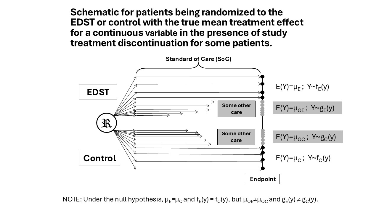
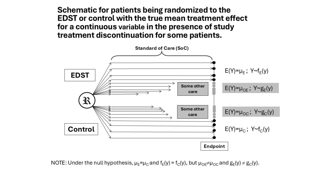
If one were interested in the “ITT effect,” then those patients who could not adhere to their randomized study treatment would be allowed to pursue whatever treatment is necessary for their best interest and their personal circumstances. The Figure below depicts this ITT approach. Patients are generally not left untreated, so presumably they will receive other care, which could be in the form of another active treatment or any medical intervention necessary for the patient (e.g., ventilation, surgery, dialysis). However, if some patients in truth would not be treated at all, the arguments that follow still hold.

In the spirit of clarity and precisions, let’s try to write the ITT effect as a parameter, an estimand to be estimated. As is common in statistical parlance, I will write the estimand as an expectation – the expected value of the clinical response related to the ITT effect. It might look something like this (if you allow me to use some casual [NOT causal] notation):

The expected (i.e., population mean) response on the experimental arm is …

where each π_i represents the proportion of patients who travel that treatment journey, for which there can be many.

So, not only are there a lot of π’s to consider, but every treatment journey will also produce a different distribution of response for Y. That’s a lot of different response distributions! The probability distribution of the HbA1c response for an experimental treatment at week 52 of a diabetes trial, for example, will be different than the distribution governing the week-52 response of a patient who discontinues the experimental treatment at, say week 26, and switches to another approved, effective anti-diabetic treatment (i.e., rescue medication). We could write a similar expectation for the control group, except the π_i’s would all be different. The treatment effect is the difference in these response expectations for experimental and control arms of the study. The true treatment effect (a parameter; the estimand) is a complex mixture distribution that is difficult to describe in anything but the most general and empirical terms. It is difficult to write it mathematically as a parameter or an expectation as is usually done in statistical analysis and estimation. As Tom Permutt wrote, “It is useful in principle to try to unmix the effects. How practical it is at present, I don’t know.” [Permutt, 2025]

If you cannot write the expectation for the treatment effect parameter that you are estimating (the estimand), how do you know if you have a good estimator/estimate of the treatment effect? How do you know if it is biased or not?

Now, for those patients who adhere to their EDST (experimental or control), one can write (or assume) a concise mathematical probability distribution function for the response Y. That is, for example, at week 52 post randomization, HbA1c is normally distributed with mean μ_E or μ_C, respectively, with common variance σ². This is difficult if not impossible to do for those who do not adhere to their randomized study medication (RSM) throughout the trial for the reasons noted above – it’s a complex mixture distribution. Furthermore, before the trial begins, we cannot even say what other treatments/interventions might be used in the care of the patient. In that sense, we cannot even say what treatment the patients in the trial will receive other than the very general “RSM + SoC,” where the SoC may vary from investigative site to site or even shift over time.

One could say that, even though I cannot explicitly define a probability distribution of the responses for those who do not adhere to their RSM, I could just say it all gets rolled up into some overall mean effect which I will call μ_OE or μ_OC for the mean response of all other treatments (O) following E and C, respectively (see the Figure above). Importantly, I will note that the other treatments/interventions that follow E may be different than those that follow C. So, it is difficult to define or even assume for study planning purposes what those parameters might be.

So, the ITT effect is the difference in responses on each arm of the study (experimental versus control) and may be written as follows:

[π₁*μ_E + (1- π₁)*μ_OE] – [π₂*μ_C + (1- π₂)*μ_OC].                                      (Eq. 1)

Obviously, since π₁ does not equal π₂ and μ_OE does not equal μ_OC, this ITT estimand is not the usual treatment effect estimand that statisticians or clinical researchers conceptualize, that is μ_E – μ_C. Thus, when a study objective states something like, “to compare HbA1c response for the experimental treatment with control response at week 52 …” and then uses a treatment policy or ITT approach (i.e., a treatment policy approach in the Addendum), the estimand implied by the selected ITT strategy is what is actually being estimated and is given in Eq 1 above, not μ_E – μ_C as might be intended in the vernacular of the objective.

As with Lipkovich et al mentioned previously in this Blog, the HOW (the strategy) implicitly or explicitly defines the WHAT. The words in the objective or other English statements in the protocol are superseded by the strategy and the mathematics derived from that strategy.

This is not new in many regards. It is well-known that the ITT effect is biased for the direct treatment effect (μ_E – μ_C). Nonetheless, some argue for the primacy of the ITT effect, and as in earlier Blogs, it is valid if the clinical question of interest is truly the initiation of EDST effect. Unfortunately, I have not seen the recognition that the implication of the ITT null hypothesis is that we are assuming a difference in the mean response for the EDST and control. It is important to recognize explicitly that

Further explanations are given in Ruberg [2026] in Chapter 9: “What Do We Mean by the Mean?” Other Addendum strategies are also examined therein, and the incongruities are not limited to the ITT or treatment policy approach.

Summary

I will go out on a limb and say that the entire purpose of ICH E9(R1) was to clarify the WHAT first and then define the HOW. I have seen recent publications and done consulting with some companies where there is some explicit description of the WHAT in an attempt to follow the ICH E9(R1) guidance. However, the WHAT is immediately countermanded when the statisticians define how incomplete data will be handled via one of the Addendum strategies. Even more complicated is when some implement different strategies for different intercurrent events, which I strongly advocate against in my book. For example, incomplete data handling strategies might be defined as follows:

I’m serious! Can anyone write the estimand for this? $\theta$ = E[Y | …] – … !!! Can anyone give a clinical language statement for this estimand? Most importantly, can any clinicians give a meaningful interpretation of this analysis approach? Such mixing of strategies implies a mixing of estimands that are extremely difficult to write as a parameters of a probability distribution or an expectation of the clinical response, Y. They are even harder to describe in plain language that has any clinical meaning.

When I describe ITT to people I know (patients, physicians, nurses, etc.), they are most often baffled. When giving an ITT effect estimate to a patient, I can say, “Look, you don’t even have to take this treatment I am prescribing, and I can say here is the treatment effect you can expect.” Some have accurately described that ITT is the effect of random assignment to a treatment, which is accurate. However, if we want to answer the question, “Does this treatment cause that outcome?” we are not interested in the “assignment” but rather the “taking” of the treatment. If there is no cause (a patient is assigned but does not take the treatment), then there can be no effect from the treatment. For there to be a causal link between the treatment and the outcome, the patient must take at least one dose of the treatment. Thus, they can initiate the treatment (in the presence of SoC or discontinue in favor of other treatments) or they can continue to take (adhere) the treatment for the duration of the trial. Understanding this distinction and deciding which is of greatest clinical interest is paramount in the estimand framework.

I am not arguing against ITT! I am arguing for a thoughtful consideration of the most meaningful clinical question to answer from a clinical trial. Both question presented herein are meaningful. In the care of a cancer patient involving a sequence of treatments/medications/interventions, I want to know the ITT effect, which is the overall prognosis. What are my chances of surviving and for how long regardless of the ups and downs and the changing of my treatment regimen(s) along the way. But I also want to know, “When I start this therapy, what can I expect to happen?” What are the benefits and side effects of THIS treatment you are planning to give me now? In the care of an Alzheimer’s disease patient, at present we know there is no cure, the treatment effect (if any) will wane, and the patient will eventually succumb to the disease. What I want to know is, “While I am taking this treatment, what can I expect to happen?” Will I maintain some level of stable cognitive ability and physical functioning? How long should I expect the treatment to work?

There are many other examples of very clinically meaningful questions that do not relate to the mere initiation of treatment effect – i.e., the ITT effect. Rarely does one size fit all, as they say. There is more to clinical research than the ITT effect. I implore the thoughtful use of the estimand framework to help guide your decision-making.

References

International Council for Harmonization (2019), “E9(R1): Addendum on estimands and sensitivity analysis in clinical trials to the guideline on statistical principles for clinical trials R9(R1),” available at https://database.ich.org/sites/default/files/E9-R1_Step4_Guideline_2019_1203.pdf.

International Council for Harmonization (1998), “Statistical Principles for Clinical Trials – E9.” Available at https://database.ich.org/sites/default/files/E9_Guideline.pdf.

Fleming TR, Carroll KJ, Wittes JT, Emerson SS, Rothmann MD, Collins S, Levin G. A Perspective on the Appropriate Implementation of ICH E9(R1) Addendum Strategies for Handling Intercurrent Events. Stat Med. 2025 May;44(10-12):e70104. doi: 10.1002/sim.70104.

Ruberg, SJ. Does This Treatment Cause That Outcome? The Science of Estimating a Treatment Effect and Why It Matters. CRC Press, Boca Raton, 2026.

Tukey J. The Future of Data Analysis. Ann. Math. Statist. 1962;33(1):1-67.

Lehmann, E. L. Theory of Point Estimation. John Wiley & Sons, 1983. p. 4

Lipkovich I, Ratitch B, & Mallinckrodt CH. (2020). Causal Inference and Estimands in Clinical Trials. Statist in Biopharm Res. 2020;12(1):54–67.