Well, I hope you are getting some new insights or learnings out of this blog because I certainly am. In my Welcome to this blog, I stated, “I am open to your comments and queries and even disagreements. I look forward to you helping me refine and improve my analytics thinking.” I received some feedback – a critique if you will – via e-mail from Oliver Keene, a very astute statistician and friendly colleague of mine, on Blog 7 – “What does p<0.05 mean anyway?” It forced me to think more deeply about how to formulate a prior for a Bayesian analysis and what is most reasonable and logical (at least to me).
[In my Welcome, I also note that I will try to make this blog accessible to those less quantitatively deep in stats/math, but I must confess that this blog will get a bit technical and formulaic. Nonetheless, I will try to point out the highlights and conclusions to those who do not want to follow the math.]
Background
[Note that those who are steeped in hypothesis testing and Bayesian thinking can skip to the next Section – The Critique. On the other hand, even if you are steeped in these concepts, you might want to read this Section so you are familiar with how I frame the problem and the terminology that I use. What is presented here is to help those who are less familiar with these concepts understand the thinking without the math.]
Let me set the stage here. In most experimental scientific investigations, a scientist has a hypothesis about the state of Nature (i.e. what is true). The null hypothesis (H0) is defined to be a “no effect” hypothesis and the alternative hypothesis (Ha) is the state of Nature that the scientist wants to prove. For example, H0 is “this new drug doesn’t work” and Ha is “the new drug works.” Thus, in standard hypothesis testing (or null hypothesis significance testing – NHST), the scientist designs an experiment, collects data, performs a statistical analysis of the data and finally wants to reject H0 in favor of Ha. In fact, what the scientist, and indeed all of us, is thinking is this:
- I have a hypothesis
- I have done an experiment to examine/test that hypothesis.
- Now that I have seen the data from that experiment, what do I believe about my hypothesis?
That is, given the data from my experiment about my hypothesis, what is the probability that Ha -my hypothesized state of Nature – is true (or equivalently H0 is false)?
In general terms, the Bayesian approach to answering this fundamental question is based on the notion
(posterior belief) is related to (prior belief) x (evidence from current data).
- “Prior belief” is all the evidence, data etc. that a scientist has that leads up to the formulation of the hypothesis and establishes the very reason and purpose for doing the experiment. All that evidence and data comes from not only the scientist’s own research efforts, but also includes any and all research done across the scientific community on the topic of investigation.
- “Evidence from the current data” is based on a statistical analysis of the data from the experiment the scientist conducted to examine/test their hypothesis.
- “Posterior belief” is the new level of confidence, belief or credibility (i.e. probability) that the research hypothesis is true (H0 is false) – e.g. “the drug works.”
Mathematically, if we let X stand for “the current data,” then statisticians write (again in general terms)
pr(H0 | X) is proportional pr(H0) * pr(X | H0) Equation 1.
One might recognize the last term in the equation above as the p-value (i.e. the probability of observing the data X given H0 is true).
With that background, in Blog 7, I argued and presented what a p-value=0.05 is “worth” using the Bayes Factor Bound and my favorite (and straightforward) formula [1] for thinking about evidence.
p1 ≤ p0*BFB/(1-p0+p0*BFB) Equation 2.
I did this by showing that regardless of the point prior p0, a p-value of 0.05 only increases the level of belief/probability by about 0.22 or less. That is, for example, a prior of p0=0.50 and a p-value of 0.05 results in a posterior probability that H0 is false of p1=0.71 or less. So, by doing an experiment that produces a p-value of 0.05 (what some call statistically significant), my level of confidence that H0 is false – or Ha is true – only moved from 0.50 (my prior) to 0.71 (my maximum posterior). I stated is a relatively small increase in probability/confidence/belief for what is traditionally considered a “significant finding.” I replicate Table 1 from Blog 7 here.
Table 1
The relationship between prior belief/probability that the null hypothesis is false
and a p-value=0.05 for testing that hypothesis using Bayes Factor Bound.
| Prior, p0 (belief, probability) | p-value | Posterior, p1 (upper bound) | Increase in “Evidence” (post – prior) |
| 0.1 | 0.05 | 0.214 | 0.114 |
| 0.2 | 0.05 | 0.380 | 0.180 |
| 0.3 | 0.05 | 0.513 | 0.213 |
| 0.4 | 0.05 | 0.621 | 0.221 |
| 0.5 | 0.05 | 0.711 | 0.211 |
| 0.6 | 0.05 | 0.787 | 0.187 |
| 0.7 | 0.05 | 0.851 | 0.151 |
The Critique
The critique I received about Table 1 goes like this, noting that I will try to be as faithful to Oliver Keene’s perspective as possible.
Suppose I have a treatment difference [that’s the difference between, say, a new drug and a placebo] that is normally distributed. Before the experiment (e.g. clinical trial), I have very little information, so I have either a weak normally distributed prior with a mean of 0 and large standard deviation or alternatively a flat prior. [For the non-mathematical, a mean of zero means the null hypothesis is true or that there is no treatment effect. Think of it as being that the treatment difference between a new drug and a placebo is zero.] Before the trial, my prior probability that the treatment difference is > 0 is 50% [i.e. it’s a coin toss as to whether the new drug works or not]. Now I run the trial and end up with a posterior probability of 97.5% that there is a treatment difference > 0 [i.e. the new drug works]. If the scientist does a NHST approach on the same data, the p-value will come out about p=0.05. So, in this case a p=0.05 has changed my prior belief from 50% to 97.5%, a large change. This is a lot different than the prior=0.50 to maximum posterior=0.71 that is shown in Table 1. What gives?
So, how did I get from a prior of 0.50 to a posterior of 0.71 using the BFB formulation of evidence and how did my critic get from a prior of 0.50 to a posterior of 0.975 with the same p-value of 0.05? This is what made me do some deeper thinking and helped me educate myself a bit better on this whole conundrum of p-values and Bayesian posterior probabilities. What I found, which may already be known by most Bayesians or others who have studied this problem for years and more deeply than I, is that the answer lies in the formulation of prior for the null and alternative hypotheses. Let’s dissect my critic’s perspective carefully.
General Response
[Warning: here is the mathematical part for those who want to skip the equations and just read the text for the concepts.]
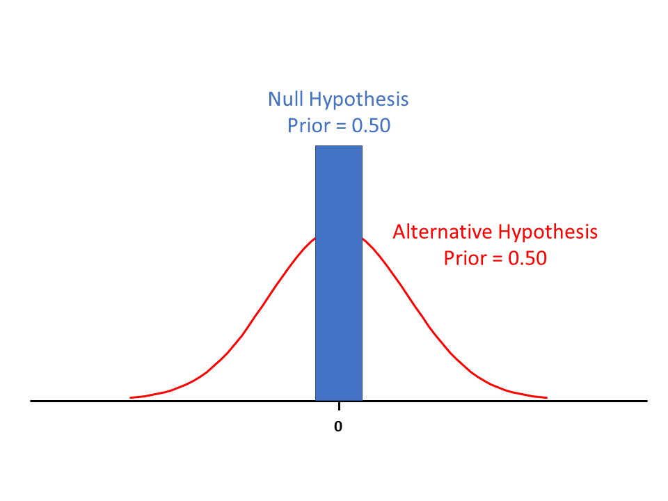
First, I have realized (more clearly) that saying that there is a 50% probability of H0 being true (or false) can be interpreted in different ways. One way is as described by my critic: with a symmetric distribution centered at 0 that could be normal (but does not have to be). The other way is using a point null hypothesis [2] and putting a probability mass near that point. I will discuss each of these formulations in turn.
Second, whenever a prior has a large standard deviation, is flat or diffuse (as some say), then pr(H0) is proportional to 1. Thus, Eq. 1
pr(H0 | X) is proportional to pr(H0) * pr(X | H0)
reduces to
pr(H0 | X) is proportional to pr(X | H0),
and the Bayesian posterior probability provides similar evidence to the p-value [a Bayesian posterior probability of 0.975 corresponds to a two-sided p-value of 0.05]. I will have more to say about the plausibility of such a diffuse/flat prior in the next Section.
Specific Response – Normally Distributed Data
For normally distributed data, the posterior mean and standard deviation can be computed analytically. I am going to use alphabetic text to describe this since this blog platform is not very amenable to Greek notation and mathematical equations.
I will first start with the comment about the problem of a normal prior and normal data to produce a normal posterior. For the sake of simplicity and consistent with the critique, let mu be the mean and sigma2 be the variance of a normal distribution. If the null hypothesis is that mu=0, and the experimental data produces a standardized test statistic = 1.96 (assuming large enough sample size to be well-approximated by a normal distribution), the two-tailed p-value is 0.05 – a significant result.
From basic Bayesian math, without loss of generality, assuming a known variance sigma2 = 1, let
mu-pr = the prior mean
sigma2-pr = the prior variance
xbar be the sample mean, and
n = sample size.
Then the posterior mean (mean-po) is
mean-po = ( (mean-pr / sigma2-pr) + (n / sigma2)*xbar ) / ( (1 / sigma2-pr) + (n / sigma2)).
For our problem mean-pr = 0 and xbar = 1.96, which allows us to simplify the above equation to
mean-po = (1.96 * n) / ( (1 / sigma-pr) + n). Equation 3
If sigma2-pr is large especially relative to sigma2 (which means we have a very diffuse prior – some might incorrectly say non-informative), then the whole equation reduces to
mean-po = 1.96.
If our posterior mean is 1.96, then what is the probability that H0: true mean = 0 is false? This is given by the posterior probability that mean-po is greater than 0 (i.e. the posterior mean … our best estimate of the true mean having seen the data) is pr(mean-po > 0) = 0.975. I believe this is what is meant in my critic’s note that a p-value of 0.05 (corresponding to a test statistic value of 1.96) produces a posterior probability of 0.975.
Of course, in Eq. 3, for any sigma-pr, as n gets large, the observed data outweighs the prior and the posterior mean converges to 1.96 and subsequent probability that the true mean exceeds 0 converges to 0.975.
The notion of a very diffuse prior (i.e. we know little about a mean value) and the posterior distribution being (nearly) equal to the distribution of the mean that comes to us through data is clearly known and stated by Berger and Sellke in their 1987 JASA paper, “Testing a Point Null Hypothesis: The Irreconcilability of P Values and Evidence” [2]. In that paper they write: “If he [the experimenter] were initially “50-50” concerning the truth of H0, if he were very uncertain about θ [the mean mu in our notatoin] should H0 be false, and if p were moderately small, then his posterior probability of H0 would essentially equal p.” (p. 114)
Now, I happen to think a prior that is a normal distribution centered at zero with the variance of the prior distribution that is much larger than the that governing the observed data (i.e. sigma2-pr >> sigma2) is quite odd. If the data is normally distributed with a variance of 1 (sigma2=1), it is like saying that I think the unknown mean could range between (say) -10 and 10, which is pretty meaningless. Certainly, we can do better than grasping at straws in the dark for how we might think about the distribution of the unknown mean. While many experiments proceed with some background knowledge and thereby justification for its conduct, there are some truly experimental hypotheses for which little might be known (e.g. think exploratory biomarker research). However, I will now present what I think is a more reasonable formulation of prior distributions.
Specific Response – Point Null Hypotheses
Another way to frame “there is a 50% probability of H0 being true (or false)” is due to Berger and Sellke in the 1987 JASA paper that discusses point null hypotheses. [I hope what follows does justification to their work.] That is, H0: θ=0, where θ represents the unknown mean of interest (e.g. a treatment effect). Of course, we know that θ precisely equal to zero is not really possible. So, they frame the problem as a null hypothesis for which θ is negligible – H0: |θ – ε|<0, and “stack” a prior probability on that, say, p0=0.50. So, they say, the probability that the null hypothesis is true is 50%, meaning that there is a probability mass of 0.50 on the very small interval |θ – ε|. That makes a lot more sense to me as a prior. In the pharmaceutical business, we might say that we have some prior belief about our null hypothesis that “the drug doesn’t work” or that “the biomarker is not predictive.” What we mean mathematically is something more akin to
θ ~ uniform (-ε, ε)
rather than
θ ~ N(0, 100).
Also, Berger et al work with the odds that’s H0 is true versus Ha is true. As such they must specify an alternative hypothesis for the distribution of θ that has (1-p0) probability. For alternative distributions, they examine all distributions, all symmetric distributions, all symmetric unimodal distributions, all normal distributions for the alternative values of θ. While I cannot claim that I can follow all the math, suffice to say that this is where the derivation of the Bayes Factor Bound (BFB) comes in. Other follow-on publications (by Berger, Sellke and friends – The Amer Stat 2001, The Amer Stat 2019 [3]) describe and refine this more leading to
posterior odds <= prior odds * BFB.
This can be unraveled to bound the posterior probability of H0 being false based as a function of the prior probability that H0 is false (i.e. Ha is true) and the BFB, which is what I have presented in my previous blogs and is shown in Eq 2 in this blog.
I will note that Berger et al deal with alternatives that are two-sided, which may not be satisfactory from a drug development perspective since we are only interested in treatments that are better than control. I do not know how this would affect the math and derivations, but one could always consider testing two-sided hypotheses, using all the math to get the BFB knowing that it is only meaningful if the treatment effect is favorable. Who cares about the probability of H0 being false if the observed response to treatment is worse than the observed response to control?! [Note that I am happy to have others comment on this two-sided versus one-sided hypothesis testing scenario.]
Final Considerations
So, frequentist NHST and Bayesian approaches give similar answers when the prior is diffuse. The answers from these approaches can diverge considerably when a different formulation of the prior is considered or when the prior for H0, p0, is considerably different than 0.50 (i.e. a coin toss) as shown in Blog 5. Which approach do I believe or follow?
My answer is this. A p-value is a precise answer (but still requiring assumptions) to the wrong question and the Bayesian posterior is an (approximate?) answer to the right question. EVERYONE wants to know, “Now that I have done my experiment and seen my data, what do I believe about my hypothesis?” The Bayesian posterior directly answers that question. As you well know, we statisticians lament when researchers interpret the p-value as that posterior probability. But that’s what researchers want and that’s what they think we as statisticians are giving them. Even when I have told researchers not to interpret a p-value that way, they usually say, “Well, but it is kind of like that.” So, we have been pulling the wool over researchers’ eyes for decades and giving them one answer that is “kind of like” what they really want and how they really interpret it. We statisticians have been giving pr(A|B) when what researchers really want is pr(B|A) … and we all wave our hands and say, “well, they are kind of the same” (which they can be when the prior is unrealistically diffuse). But there are too many situations when such priors are not diffuse. I have found the use of the BFB and Eq. 2 has consistently provided me with answers (i.e. probabilities) that are (a) more aligned with my intuition, (b) more logical based on available scientific evidence and (c) more predictive of future experimental results.
By this last point (c) I mean that Bayesian probabilities calculated by Eq 2 give a more realistic assessment of the probability of success of future experiments than relying on a p-value<0.05, which is most often used to convey that there is a significant finding and one that is likely to reflect some reality that H0 is false. If you don’t believe me, you only have to read a tiny bit of the vast literature on the “crisis of reproducibility” in scientific research to see that an over-reliance on p-values has led our scientific thinking astray as much or, in some cases, even more often that it has helped.
But there is another argument to support my assertion in (c) that I can offer – the success rate of investigational treatments in pharmaceutical research. In the most comprehensive study of the success rates of investigational treatments in the pharmaceutical industry [4], Hay et al examined 4,451 treatments and 5,820 phase transitions over a period of 2003-2011. They found that overall there was about a 20% chance of approval of a treatment when starting Phase 2 of clinical development (see their Table 4). So, let’s take that as our prior since it is based on a very large sample size. As an insider to several pharma companies over several decades, I can say that pharmaceutical companies act on Phase 2 results that are significant (p=0.01-0.05 is typical) and believe that there is a high likelihood of success in Phase 3 with such significant Phase 2 findings. If we use Eq 2, inputting p0=0.20 and p-values of 0.05, 0.025 and 0.01 for a successful Phase 2 study, the resulting posterior probabilities that are predictive of future success are, respectively, 0.38, 0.50 and 0.67. These posterior probabilities are very much in line with the “Likelihood of Approval (LoA)” presented in the Hay et al paper based on many hundreds of investigational treatments. Thus, a Phase 2 p-value=0.05, which is viewed as very indicative that a “drug works” (i.e. H0 is false), and certainly a p-value=0.01, which is thought to be almost a “slam dunk” in terms of Phase 3 success, are actually not very good indicators of future success in Phase 3. Alternatively, the Bayesian posterior probability, even calculated somewhat crudely (using Eq 2) over a large sample of investigational treatment, is much more in line with the observed success rates in Phase 3 and approval.
Finally, hypothesis testing is akin to proof by contradiction in mathematics, though in mathematics, the answer is absolutely true or false. We start with a premise or statement and we use known, valid mathematical steps until we get a known contradictory (or confirmatory) answer. Then we conclude that the premise is false (or true depending on the answer). In statistics we put a probability on the answer – aka a p-value. We have a null hypothesis, collect data and analyze it in known valid ways to get a probability answer. We infer H0 or Ha depending on the size of that probability. Bayesian approaches are more like direct proof. They make a probability statements directly about the question of interest – how likely is it that H0 or Ha is true? As noted above, I prefer to answer the right question, even if it is approximate due to their being at least some element of subjectivity to the prior. Then again, any researcher with any experience interprets a p-value with some level of subjective evaluation. If a statistically significant finding (p<0.05) is a big surprise or against the scientific orthodoxy, then it is viewed skeptically because the researcher interprets it with their own subjective and IMPLICIT prior. “I am not sure I believe that result.” Why not make the prior EXPLICIT and do the real work to answer the question of interest?!
References
- Sellke, T., Bayarri, M. J., Berger, J. O. Calibration of p values for testing precise null hypotheses. The Amer. Statist. 55, 62-71 (2001).
- Berger, J. O., and Sellke, T. (1987), “Testing a Point Null Hypothesis: The Irreconcilability of p Values and Evidence,” Journal of the American Statistical Association, 82, 112–122.
- Benjamin, D., and Berger, J. (2019), “Three Recommendations for Improving the Use of p-Values,” The American Statistician, 73, 186-191.
- Hay, M., Thomas, D. W., Craighead, J. L., Economides. C., and Rosenthal. J., (2014). “Clinical Development Success Rates for Investigational Drugs.” Nature Biotechnology, 32 (1): 40-51.
